I am often tempted to try the programming language Julia for scientific computing. It promises fast execution and relative ease of operation: it can run in a Jupyter notebook and is dynamically typed. Furthermore, it has a growing number of well-reviewed packages, including for differential equations and machine learning. In this blog-post I am going to benchmark Python’s SciPy module against Julia for solving the matrix equation (Ax = b), where A is a sparse matrix. This equation is ubiquitous in science and engineering. Here it arises from numerically solving partial differential equations (PDEs) by the finite difference method.
Specifically, I am going to solve the Poisson equation in 2-d, with an analytic solution for comparison. Each row of the Poisson equation matrix in 2-d contains a diagonal term, 4 off-diagonal terms and a lot of zeros. If there are Nx (Ny) grid points in x (y), the matrix has dimensions (Nx*Ny, Nx*Ny). I remember being amazed at the speed-up achieved by treating this matrix as sparse (e.g. using scipy.sparse.linalg.spsolve vs. scipy.linalg.solve). So here I limit myself to sparse matrices. I will compare direct solvers and also a conjugate gradient iterative solver. The Jupyter notebooks are available in a GitHub repository.
The Poisson equation
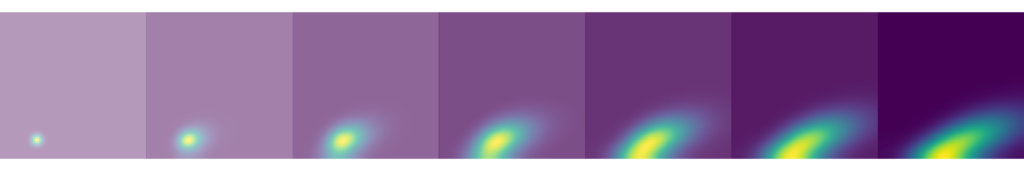
I described the Poisson equation, its discretisation and the use of a model solution in a previous blog-post. The methodology and analytic solution here are identical so I will not repeat the discussion. In the figure below I show a comparison of the analytic solution with the solution achieved by a direct solver in Python. Visually they are similar, which is good. When a more precise comparison is needed, as towards the end of this article, we use the L2 norm of the two solutions.


Benchmarking
I call several functions in the Python and Julia scripts. First, generate the source term for the Poisson equation. Second, populate the sparse matrix. Third, solve the matrix equation. And finally, wrap the solution of the matrix equation into an array so it can be easily plotted. I benchmark only the third part of the flow (i.e. the solution of the matrix equation). At least for large grid dimensions, it is the most time-consuming part of the calculation. The mean runtime of the relevant Python function is determined by the %timeit magic command within a Jupyter notebook. In Julia, the @benchmark macro is used. In both cases the average runtime over many runs is calculated and the compile time of the Julia code is not included.
First, let us take a look at the performance of the direct solvers (figure below). These are ‘scipy.sparse.linalg.spsolve‘ in the case of Python and simply the ‘\’ operator (multiple dispatch is occurring under the hood) for Julia. Perhaps surprisingly, the performance isn’t too different, with Julia being slightly faster at the largest number of grid points.
It is more time-efficient to use an iterative solver. In this case I use the conjugate gradient solvers (scipy.sparse.linalg.cg and IterativeSolvers.cg), since it is known we have a positive definite matrix. In both cases, I set the relative tolerance to 1e-8. And here we do notice that Julia is faster than Python for small grid dimensions. However, at the larger grid dimensions, that would be used in an actual simulation, Python and Julia are again comparable.

Has there been a reduction in accuracy in going to an iterative solver? Let’s look at the L2 norm to check (figure below). Actually for all numbers of grid points and for all methods the L2 norm is essentially identical. This shows that the truncation error (the error from discretising the PDE) dominates and there is no accuracy penalty due to using an iterative solver. Note that a rather small relative tolerance was used in the case of the iterative solvers.

Conclusions
The performance of the Python (SciPy) and Julia methods for solving a sparse matrix equation are comparable. This is true both for the direct solvers and iterative solvers. At least for the time being, I will continue to write PDE solvers in Python.